Hypotheses Testing — How is it useful in machine learning?
Hypothesis testing is a way to tell if some belief you have of the population is likely to be true or false.
Let’s say you have an email spam detector and what it does is it determines if a given email is Not Spam or Spam. And Not Spam is when an email is not spam. And by default, we’re going to assume that all the emails are Not Spam. And the reason for this is that it’s much worse to delete a good email than to accidentally put a spam email on our inbox. So our base assumption is going to be that an email is Not Spam. That’s going to be called the null hypothesis. It’s the base assumption when we assume safely that nothing is happening. The null hypothesis is called H0. We also have alternate hypothesis which is H1. One important characteristic of the null and alternative hypothesis is that they are mutually exclusive.
The key is to designing a good set of hypothesis. There’s a lot of evidence that shows that the email is spam. Then the null hypothesis is rejected and the alternative hypothesis that the email is spam is accepted as true.
If the evidence gathered is not enough to show that the email is spam, then you can reject the null hypothesis. However, that does not mean that the email is not spam, only that we don’t have enough evidence to show that the email is spam.
The null hypothesis is the baseline and the alternative hypothesis represents the competing statement.
There can be scenarios where this can go wrong, they are called Type 1 error (False Positive) and Type II error (False Negative).

Sending a regular email to spam is worse than not sending a spam email to the regular inbox. Type I error is more significant than the Type II error.
What is the greatest probability of type I error you are willing to tolerate?
The maximum probability of type I error is called the significance level and is usually denoted by the Greek letter alpha. Of course, since it’s a probability, it can only take values between 0 and 1. If alpha is 0, it means that whatever evidence you get, the email is always considered to be not spam. In that case, you never get a type I error. On the other end, if the significance level is 1, that means every email is considered spam. And in this case, every time you get a not spam email, you will be making a type I error. Of course, both extremes are terrible decision makers. What you want is something that is able to define if an email is spam or not and has as few type I errors as possible.
However, as you saw, this error can never be made 0, so a typical value to consider is 0.05 for your significance level. This means that on average, you will decide that a not spam email is spam 5% of the time. Another value usually encountered is alpha equals 0.01. As we said, you want alpha to be as small as possible. But however, there’s a small catch. If you reduce the probability of a type I error too much for a fixed number of samples, then you’re increasing the type II error. This is what happens when we thought of the alpha equals 0 scenario. To give the proper definition of significance level, it is the maximum probability of committing a type I error, which is the same as the maximum probability of rejecting H0 when H0 was actually true. The value of alpha is your design criterion for this test. This means that alpha will determine a threshold to decide if you should reject H0 or not based on your sample.
For this hypothesis testing, it is always important to have data quality. It should be reliable. The sample should represent the population and it should be randomized so it does not have any bias. Also, sample size is important.
If our null hypothesis is based on the sample mean then it is Test Statistics and on other hand we have observed statistics.

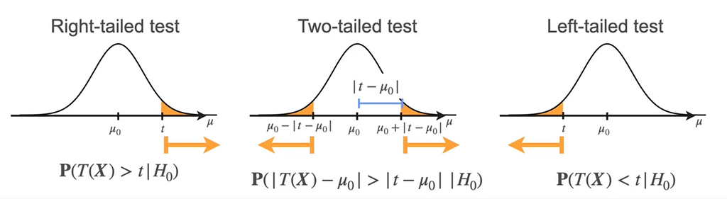
In general, we have 3 types of hypothesis
- Right tailed test — The alternate hypothesis is right side or greater than the null hypothesis
- Left tailed test — The alternate hypothesis is left side or less than the null hypothesis
- Two tailed test — The alternate hypothesis is either left or right tailed but not equal to null hypothesis
p-value
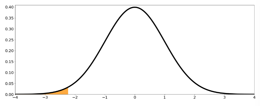
A p-value is the probability assuming H_0 is true, that the test statistic takes on a value as extreme as or more extreme than the value observed.
Suppose now that the standard deviation that there was no change throughout the years. We are assuming that the standard deviation is known. How likely was your sample if H0 is true? If the answer is very unlikely, then reject H0. Consider now the right-tail test for the mean of a population with the Gaussian distribution.
Our goal is to make a decision with the type 1 error probability of no more than the significance level alpha which is 5%. The maximum probability of incurring a type 1 error is below the 0.05 threshold you are willing to tolerate. It then makes sense to reject the null hypothesis. The probability used here is nothing but the p-value.
While T(X) is the test statistic and t is the observed statistic.
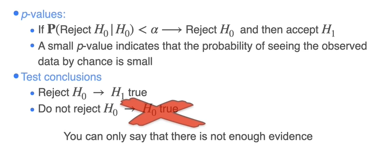
- If the p-value is less than α (significance level), then you reject the null hypothesis.
- The p-value represents the probability of observing the data or more extreme results under the assumption that the null hypothesis is true.
- A smaller p-value indicates stronger evidence against the null hypothesis.
We can apply standardization using Z statistic considering we have sample of 10 and 3 is the standard deviation.

We reject thee null hypothesis if H0 is less than the significance level. But what is the extreme sample you could get that you would still reject H0?
This is called the critical value where p-value is equal to significance value. Notice that it depends on the value that you choose for Alpha. Different Alpha’s determined different critical values. The critical value is usually referred to as K Alpha to emphasize this dependency. One cool thing about critical values is that any observed statistic which is more extreme than your critical value, will always achieve a p-value of Alpha or less. You can create a decision rule based on the critical value.
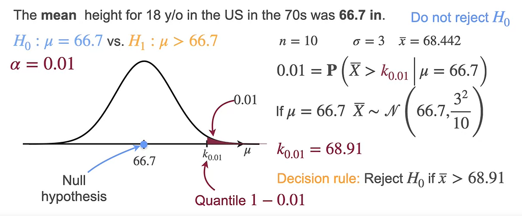
Consider this example, where the mean is 66.7 and the alternate hypothesis is greater than 66.7. If the K value is 0.01 then the critical value would be 68.91 and we reject the null hypothesis if the mean is greater than 68.91.
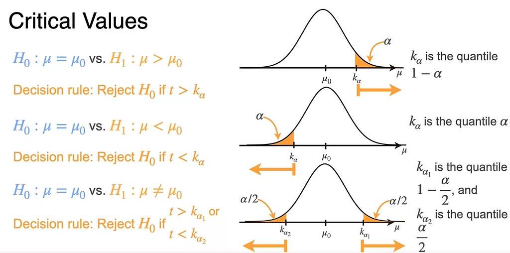
For right-tail test, K α is the value that under the null hypothesis lives an area of Alpha to it’s right. That means that the critical value is the quantile, 1- α of the statistic distribution when a H0 is true. Decision rule becomes rejected H0 if the observed statistic T is greater than the critical value.
For left-tailed test, the critical value will be the one that leaves an area of α to the left so that it corresponds to the quantile α. In this case, the decision rule is to reject the null hypothesis if the observed statistic is smaller than the critical value.
In two-tailed tests, the probability of error needs to be divided between the two tails of the distribution. Which means you will need to find two critical values K α one which leaves an area α 2 to it’s right, and K Alpha two which looks an area of Alpha two to its left. They correspond to the 1- α/2 and the α/2 quantiles respectively. You will now reject H0 if the observed statistic is greater than K Alpha one or smaller than K Alpha two.
To sum up critical values,
- we can define the critical value in advance since you don’t need the sample to get it, you only need to know the design conditions like the sample size and any information you might need about the distribution of the population you’re studying.
- It is very important that the P-value method and the critical value method must always lead you to the same conclusion.
- As we mentioned, with critical values, you can define the decision criteria beforehand and then make the decision once you have your data. This makes it possible to determine the type II error probabilities. Since you have a clear decision rule that does not depend on the observations, you can find the probability of making a type II error very easily.
Powe of the Test —
Probability of type II errors is usually called beta. A very interesting thing is that the probability does not depend on the observed sample, only on the significance level that you chose for the test. But you can get the type II error probability for any value on mu in the alternative hypothesis.
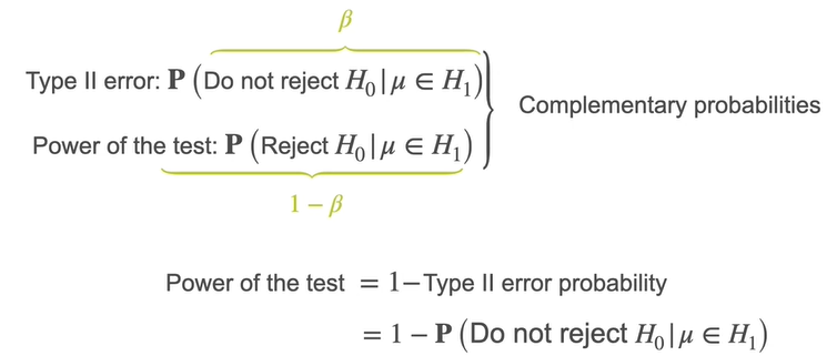
You can define beta for as many values as you want. Now, you should have a better understanding about type I and type II errors, but many times you want to characterize the chances of actually making a good decision. In particular, it is important to focus on this quadrant of the table, where you are making the right call by rejecting the null hypothesis. This information is gathered in the power of the test, which is a function that tells you for each possible value of the population, meaning the alternative hypothesis, the probability of rejecting H0. Remember that the type II error probability is the probability of not rejecting H0, when H0 is not true. This was called beta. Now, we have introduced the concept of the power of the test which is the probability of making the right decision, and rejecting the null hypothesis when it’s not true. These probabilities complement each other, so the power of the test can be written as 1-beta. To sum up for each value of mu in H1, the power of the test is 1- the probability of making a type II error.

This is what a typical power of the test looks like for a right sided test. At the very left of the plot you have mu equals 66.7, and the height of the graph is exactly alpha, since it’s the probability of rejecting H0 for that particular value of mu.
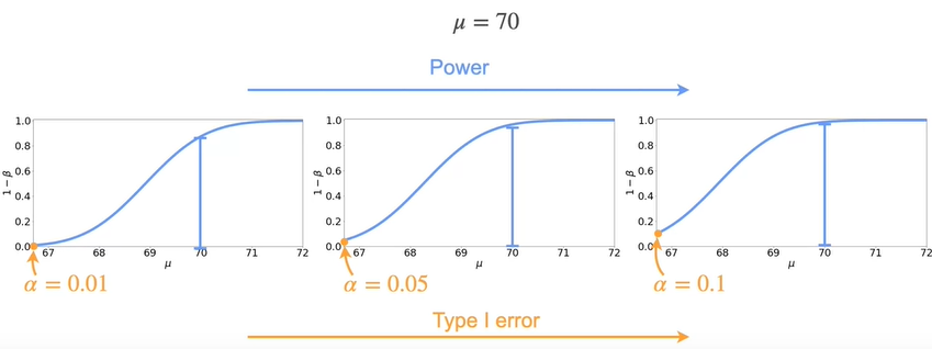
Let’s see how the power of the test looks for three different alpha values. On the left you have the power of the test for alpha with 0.01. Next for 0.05, which is the 1 from the previous slide. And finally, you have the power of the test for a significance level of 0.1. From left to right you have an increasing alpha, which is the type I error. Now consider the value of the function for mu equals 70. It turns out that as the value of alpha increases, so does the power of the test for mu equals 70. This is true for every value in the curve.
Steps for Performing Hypothesis Testing
State your Hypotheses
- Null Hypothesis — The baseline
- Alternate Hypothesis — the statement you want to prove
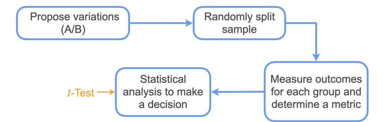
Design your test
- Decide the test statistic to work with
- Decide the significance level
Compute the observed statistic
Reach your conclusion
- If the p-value is less than the significance level reject H0
Summary
The above theory works for the standard deviation is known.
What if we do not know standard deviation?
We use t-distribution if the standard distribution is not known. We take the sample standard distribution s

The probability distribution looks bell-shaped like the standard gaussian distribution but with heavier tails that account for uncertainty introduced with the standard estimation.

It has 1 parameter which is degree of freedom v which controls how heavy the tails are


T- statistic is used when
- The population has a Gaussian distribution
- But you don’t know the variance.
Testing for Population proportion
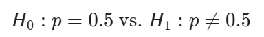
Imagine that you have a coin, but you don’t know whether it’s fair or not. The proportion you are interested in is p=P(H). A possible set of hypothesis for this problem is
Imagine you toss the coin 20 times, of which 7 turned out heads. Your random sample consists in one random variable X=”number of heads in 20 coin flips”, which has a Binomial(20,p) distribution. A good estimation for the proportion is the relative frequency of heads:

Remember that under certain conditions, the Central Limit Theorem states that
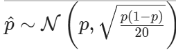
or equivalently

Z will be your test statistic. If H0is true (p=0.5), then your test statistic becomes

Consider a significance level α=0.05. Then to make a decision you need to get the p-value for your observed statistic. With the observed sample x=7, the observed statistic is

The p-value is then the probability that Z>∣z∣ or X<−∣z∣:


Conclusion: since the p-value is bigger than the significance level of 0.05, you do not have enough evidence to reject the null hypothesis that p=0.5.
Let us generalize this
- p is the population proportion of individuals in a particular category (i.e. probability of the coin landing heads)
- p0 is the population proportion under the null hypothesis (i.e. p0=0.5)
- x is the observed number of individuals in the sample from the specified category (i.e. number of heads)
- n is the sample size (i.e. number of coin toss)
- p^=x/n is the sample proportion for the observed sample x.
Then,

is the test statistic for comparing proportions, and

is the observed statistic.
Depending on the type of hypothesis, you have different expressions for the p-value:
Right-Tailed Test:


Left-Tailed Test:

Two-tailed test:


For this results to be valid, the following conditions need to be satisfied:
- The population size needs to be at least 20 times bigger than the sample size. This is necessary to ensure that all samples are independent. This condition is not needed in situation like the coin toss, where independence is inherent to the experiment.
- The individuals in the population can be divided into two categories: whether they belong to the specified category or they don’t
- The values np0>10 and n(1−p0)>10. This condition needs to be verified so that the Gaussian approximation holds when the assumption that H0 is true.
Two Sample t-Test
Two sample hypothesis testing is going to tell us how to compare samples on different populations.
Assumptions —
- All people in the sample from the two groups are different
- Each person in the both samples are independent
- Populations are normally distributed

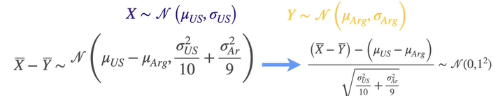
Suppose we have 10 samples in US and 9 samples in Arg

We can standardize the difference between X bar and Y bar.
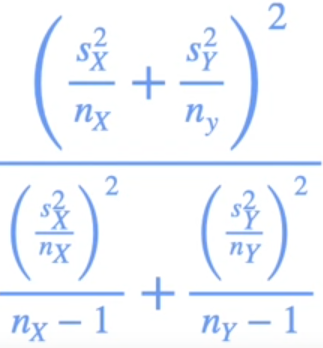
If we do not know the standard deviations we can replace with the sample standard distribution but we use degrees of freedom.

The degrees of freedom is given by
Two sample t-test for proportions
Imagine you want to compare the proportion of households that own a car in Chicago (p1) with the proportion of households that do in New York (p2). Note that p1 and p2 are population proportions.
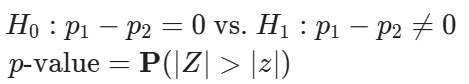
A possible set of hypothesis for this problem is

Consider for this test a significance level of 0.05
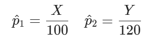
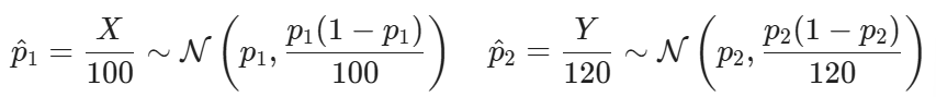
Suppose you randomly sample n1=100 households from Chicago, 62 of which own a car, and n2=120 households from New York, 58 of which own a car.
Defining X=”number of households that own a car in Chicago” and Y=”number of households that own a car in New York: , a good approximation for p1and p2 are
Naturally, a good approximation for
In order to get a good test statistic, you need to find the distribution of Δ^. First, note that in n1and n2 are big enough, which in this case they are.
so that

If H0 is true, then p1=p2=p. This simplifies the expression quite a bit! In this case,

Standardizing, you get that

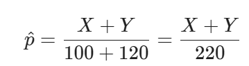
Unfortunately, this statistic is not good enough, because even if H0 is true, you do not know the value of p. However, you can replace it by the aggregated sample proportion. If H0 is true, and p1=p2=p, then X∼Binomial(100,p) and Y∼Binomial(120,p), so you can use both samples to get a better estimate of p:
Replacing p with p^ you finally get the test statistic
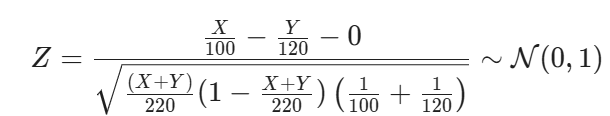
To simplify the expression even further,

With the observations you have (x=62, y=58), the observed statistic results z=2.0271. Since you are proposing a two-sided test, then the p-value is the probability that Z>2.0271 or Z<−2.0271:

Conclusion: Since the p-value is smaller than the significance level (0.05), then you reach the conclusion that you have enough evidence to reject the null hypothesis, and accept that the two population proportions are different
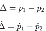
Generalizing this example,
You have two populations or groups you want to compare.
- p1−p2, is the difference in the population proportion between two groups. (i.e. the difference in the proportion of households that own a car in Chicago and New York)
- x is the observed number of individuals in the sample from the specified category from one of the groups(i.e. number households that own a car in Chicago )
- y is the observed number of individuals in the sample from the specified category from one of the groups(i.e. number households that own a car in New York )
- n1 is the sample size for group 1 (sample size from Chicago)
- n2 is the sample size for group 2 (sample size from New York)
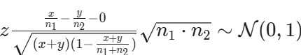
Then the test statistic is

and the observed statistic is
Depending on the type of hypothesis, you have different expressions for the p-value:
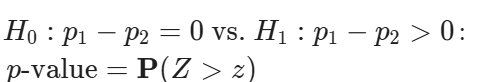
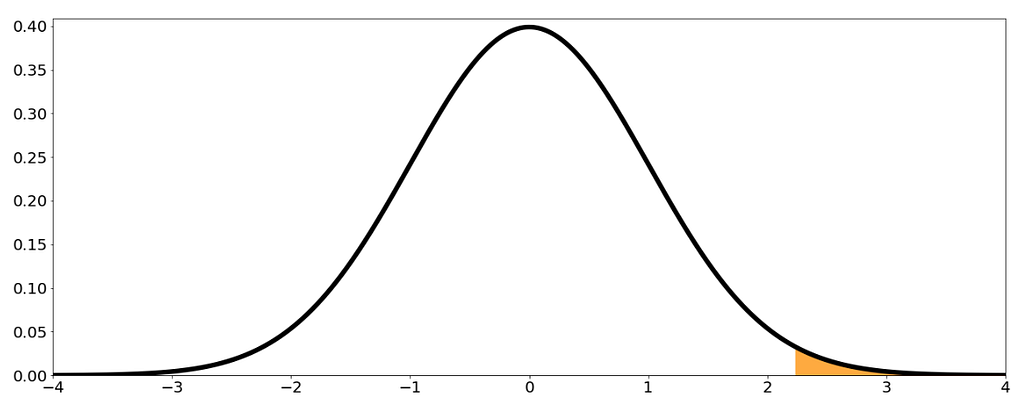
Right-Tailed Test
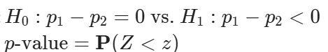
Left-Tailed Test

Two-tailed test

For this results to be valid, the following conditions need to be satisfied:
- There are two simple random samples that are independent from one another. This means that you have one sample from population 1, and another from population 2, and that the samples are independent between both groups.
- Each population size needs to be at least 20 times bigger than the sample size. This is necessary to ensure that all samples are independent.
- The individuals in each sample can be divided into two categories: wither they belong to the specified category or they don’t
- Both sample sizes need to be at least 10. This condition needs to be verified so that the Gaussian approximation holds when the assumption that H0 is true.
Paired t-Test
You learned about two sample t-test where you wanted to compare two populations where the two groups being compared were independent. There’s another situation where you also have two groups, but they are not independent.
Now you are interested in the difference between pair of samples. If the sample size in two groups is 10 then
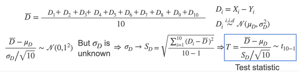
D is the difference between corresponding pairs in two groups.
Now that we learnt all about Hypothesis Testing, we would now see how is it used in Machine Learning
A/B Testing
A/B testing is a methodology for comparing two variations (A/B)
Happy Learning!!
References : DeepLearning.ai