ML Series — What if you have multiple features to predict the best model: Multiple Linear Regression
Linear Regression is one of most powerful Supervised machine learning algorithm. To know more about it —
ML Series — Linear Regression-Most used Machine Learning Algorithm: In simple Terms
We have predicted the model based on one parameter or feature that is house price based on the square feet. But in real time, we have other factors that determines the price of the house.
Let us consider we have other features also affect the price. Along with Size in square feet, Number of bedrooms, Number of floors, Age of the home in years. Let us use x1, x2, x3 and x4 to denote these features. or we can use Xj where j = 1, 2, 3, 4. and n to denote the number of features. In this case, n = 4. X(1) denotes the first training values and X(n) denotes the nth value.

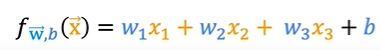
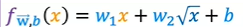
This is the function with multiple features and a bias
The vector notation of the W and X gives

where W and X are the vectors which is the row matrix of the values.
Vectorization
Using vectorization, it makes the code shorter and make it run much more efficiently. Learning how to write vectorized code will allow you to also take advantage of modern numerical linear algebra libraries, as well as maybe even GPU hardware that stands for graphics processing unit. This is hardware objectively designed to speed up computer graphics in your computer, but turns our can be used when you write vectorized code to also help you execute your code much more quickly.
We can use python library Numpy to do the operations on the array

This is the representation when we do not use vectorization and the python code is
f = 0
for j in range(n):
  f = f + w[j] * x[j]
f = f + b

This is the expression when we use vectorization which is dot product of W and X where the python implementation would be
f = np.dot(w,x) + b
How does computer makes vectorized code run faster?
Consider the example above where python code for non vectorized code. We have a for loop where j ranges from 0 to n. This piece of code performs the operations one after other. On the first timestamp we can mark as t0. It first operates on the values at index 0. At next time step, it calculates on the next timestamp and so on until all the steps are done.
In contrast, Numpy is implemented in computer hardware with vectorization. The computer can get all the values of the vectors w and x, in a single-step, it multiples each pair of w and x with each other all at the same time in parallel. Then after that, the computer takes these n numbers and uses specialized hardware to add them altogether very efficiently, rather than needing to carry out distinct additions one after another to add up to these n numbers.
This means that codes with vectorization can perform calculations in much less time than codes without vectorization.
This matters more when you are running algorithms on large data sets or trying to train large models, which is often the case with machine learning. That’s why being able to vectorize implementations of learning algorithms, has been a key step to getting learning algorithms to run efficiently, and therefore scale well to large datasets that many modern machine learning algorithms now have to operate on.
Let us say we have weights w1 to w16 and derivatives d1 to d16. Now for finding the Gradient descent, we have wj = wj — 0.1 * dj for j = 1..16
Without vectorization

With Vectorization we have

Gradient Descent for Multiple Linear Regression
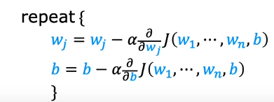
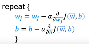
We know that the gradient descent for the Linear regression is
If you look at the vector representation we get
For single feature, we know that expanding the above formula of partial derivative of J(w, b), it looks like
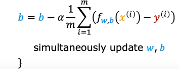
This is how we simultaneously update the values of w and b to find the minimum.
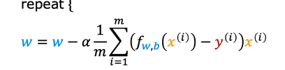
When we have multiple features

As you can see the difference is now w has been changed to w1 and x to x1 which means you are calculating for each feature. We get for wn and b

Feature Scaling
This is one method which helps gradient descent to work much faster. consider an example of the house prices based on 2 features which are square feet and number of bedrooms. If you observe the features, feature 1 value ranges from 0–2000 while the second feature ranges from 0–5. Suppose we take the weights as w1 = 50 and w2 = 0.2 with b = 50. The total would be $100,0000k which is very far away from the actual price $500,000. Now consider the other way w1 = 0.2 and w2 = 50 with b = 50. This gives the value of $500,000 which makes more sense.
Likewise, when the possible values of the feature are small, like the number of bedrooms, then a reasonable value for its parameters will be relatively large like 50. So how does this relate to grading descent? Well, let’s take a look at the scatter plot of the features where the size square feet is the horizontal axis x1 and the number of bedrooms exudes is on the vertical axis. If you plot the training data, you notice that the horizontal axis is on a much larger scale or much larger range of values compared to the vertical axis.

With small increase in the w1 there might be major changes in the values. So to have uniformity, we can map the both features between 0 and 1 which gives the contour plot more uniform
when you have different features that take on very different ranges of values, it can cause gradient descent to run slowly but re scaling the different features so they all take on comparable range of values. because speed, upgrade and dissent significantly.

In addition to dividing by the maximum, you can also do what’s called mean normalization. You start with the original features and then you re-scale them so that both of them are centered around zero. Whereas before they only had values greater than zero, now they have both negative and positive values that may be usually between negative one and plus one.
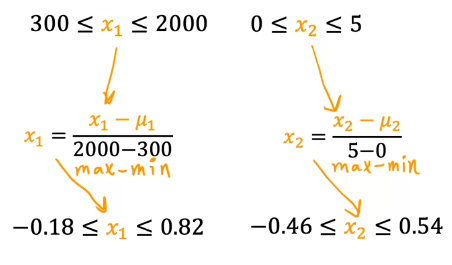
To calculate the mean normalization of x_1, first find the average, also called the mean of x_1 on your training set, and let’s call this mean Mu_1, with this being the Greek alphabets Mu. For example, you may find that the average of feature 1, Mu_1 is 600 square feet. Let’s take each x_1, subtract the mean Mu_1, and then let’s divide by the difference 2,000 minus 300, where 2,000 is the maximum and 300 the minimum, and if you do this, you get the normalized x_1 to range from negative 0.18–0.82. Similarly, to mean normalized x_2, you can calculate the average of feature 2. For instance, Mu_2 may be 2.3. Then you can take each x_2, subtract Mu_2 and divide by 5 minus 0. Again, the max 5 minus the mean, which is 0. The mean normalized x_2 now ranges from negative 0.46–0 54. If you plot the training data using the mean normalized x_1 and x_2,it might look like this.
There’s one last common re-scaling method call Z-score normalization. To implement Z-score normalization, you need to calculate something called the standard deviation of each feature. if you’ve heard of the normal distribution or the bell-shaped curve, sometimes also called the Gaussian distribution, this is what the standard deviation for the normal distribution looks like. To implement a Z-score normalization, you first calculate the mean Mu, as well as the standard deviation, which is often denoted by the lowercase Greek alphabet Sigma of each feature.
For instance, maybe feature 1 has a standard deviation of 450 and mean 600, then to Z-score normalize x_1, take each x_1, subtract Mu_1, and then divide by the standard deviation, which I’m going to denote as Sigma 1. What you may find is that the Z-score normalized x_1 now ranges from negative 0.67–3.1.

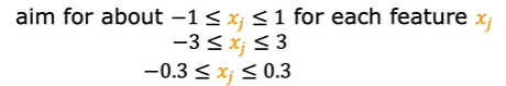
As a thumb rule, we will aim for -1 to 1 but if it ranges from different values, it is all acceptable ranges
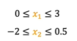
The above ranges does not require rescaling but if the values are

This should be rescaled. As the values above are either large range or small range it is recommended to do rescaling and this makes the gradient descent is reaching the minimum faster.
How will we know if gradient descent is converging?
We knew that, the key choice of learning rate alpha. If we plot the graph with the number of iterations of gradient descent and cost function on y-axis. we get the plot as
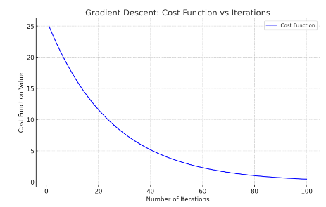
This curve is also called as learning curve. In this curve, after reaching 40 iterations, you reach the cost function of 5. Looking at this graph helps you to see how your cost J changes after each iteration of gradient descent. If gradient descent is working properly, then the cost J should decrease after every single iteration. If J ever increases after one iteration, that means either Alpha is chosen poorly, and it usually means Alpha is too large, or there could be a bug in the code. Another useful thing that this part can tell you is that if you look at this curve, by the time you reach maybe 60 iterations also, the cost J is leveling off and is no longer decreasing much. By 100 iterations, it looks like the curve has flattened out. This means that gradient descent has more or less converged because the curve is no longer decreasing. Looking at this learning curve, you can try to spot whether or not gradient descent is converging.
We can find if the gradient descent is converging for the model by automatic convergence test. Let’s let epsilon be a variable representing a small number, such as 0.001 or 10^-3. If the cost J decreases by less than this number epsilon on one iteration, then you’re likely on this flattened part of the curve that you see and you can declare convergence. Remember, convergence, hopefully in the case that you found parameters w and b that are close to the minimum possible value of J. I usually find that choosing the right threshold epsilon is pretty difficult.
Choosing Learning Rate
we know that choice of learning rate is crucial, because if the alpha is small it will run very slowly and if it is too large it may not even converge.
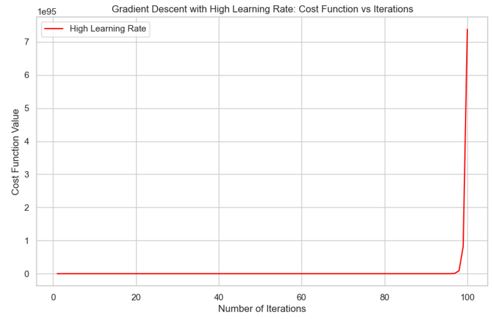
How do we know that the learning curve is too large?
The learning curve is either increasing or constant and then increases suddenly with number of iterations. Sometimes it is up and down and it is clear indication that learning rate is high. with each iteration there should be minimum value and it should be less than previous. But there can also be situation where it is constant and increases suddenly.
We can also choose the very very small learning rate and see if the value of J is decreasing. If it is not, then check the code for any bug. We can also choose first small value and then multiply by certain amount and see the value of learning curve. If the curve is good which means learning rate is not too high or low.
Feature Engineering
The choice of features can have a huge impact on your learning algorithm’s performance. In fact, for many practical applications, choosing or entering the right features is a critical step to making the algorithm work well.
Let’s take a look at feature engineering by revisiting the example of predicting the price of a house. Say you have two features for each house. x1 is the width of the lot size of the plots of land that the house is built on. This in real state is also called the frontage of the lot, and the second feature, x2, is the depth of the lot size of, lets assume the rectangular plot of land that the house was built on.

Given these two features, x_1 and x_2, you might build a model like this where

where x1 is the frontage or width, and x2 is the depth.
This model might work okay. But here’s another option for how you might choose a different way to use these features in the model that could be even more effective. You might notice that the area of the land can be calculated as the frontage or width times the depth.

You may have an intuition that the area of the land is more predictive of the price, than the frontage and depth as separate features. You might define a new feature, x3, as x1 * x2. This new feature x3 is equal to the area of the plot of land. With this feature, you can then have a model
so that the model can now choose parameters w1, w2, and w3, depending on whether the data shows that the frontage or the depth or the area x3 of the lot turns out to be the most important thing for predicting the price of the house. What we just did, creating a new feature is an example of what’s called feature engineering, in which you might use your knowledge or intuition about the problem to design new features usually by transforming or combining the original features of the problem in order to make it easier for the learning algorithm to make accurate predictions. Depending on what insights you may have into the application, rather than just taking the features that you happen to have started off with sometimes by defining new features, you might be able to get a much better model. That’s feature engineering. It turns out that this one flavor of feature engineering, that allow you to fit not just straight lines, but curves, non-linear functions to your data.
Polynomial Regression
The polynomial regression will let you fit the curves, non-linear functions to your data.
Let’s say you have a housing data-set that looks like this, where feature x is the size in square feet.
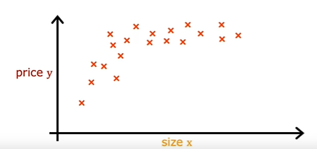
It doesn’t look like a straight line fits this data-set very well. Maybe you want to fit a curve, maybe a quadratic function to the data like this
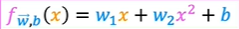
which includes a size x and also x squared, which is the size raised to the power of two. Maybe that will give you a better fit to the data. But then you may decide that your quadratic model doesn’t really make sense because a quadratic function eventually comes back down. Well, we wouldn’t really expect housing prices to go down when the size increases. Big houses seem like they should usually cost more. Then you may choose a cubic function where we now have not only x squared, but x cubed.

Maybe this model produces this curve here, which is a somewhat better fit to the data because the size does eventually come back up as the size increases. These are both examples of polynomial regression, because you took your optional feature x, and raised it to the power of two or three or any other power. In the case of the cubic function, the first feature is the size, the second feature is the size squared, and the third feature is the size cubed.
I just want to point out one more thing, which is that if you create features that are these powers like the square of the original features like this, then feature scaling becomes increasingly important. If the size of the house ranges from say, 1–1,000 square feet, then the second feature, which is a size squared, will range from one to a million, and the third feature, which is size cubed, ranges from one to a billion. These two features, x² and x³, take on very different ranges of values compared to the original feature x. If you’re using gradient descent, it’s important to apply feature scaling to get your features into comparable ranges of values. Finally, just one last example of how you really have a wide range of choices of features to use. Another reasonable alternative to taking the size squared and size cubed is to say use the square root of x. Your model may look like
The square root function looks like this, and it becomes a bit less steep as x increases, but it doesn’t ever completely flatten out, and it certainly never ever comes back down. This would be another choice of features that might work well for this data-set as well.
By using feature engineering and polynomial functions, you can potentially geta much better model for your data.
Scikit-learn is a very widely used open source machine learning library that is used by many practitioners in many of the top AI, internet, machine learning companies in the world.
Happy Learning!!