We know that transformers can be fine-tuned to produce great results on wide range of tasks. In many situations accuracy is not enough bue need fast inference. Alternative to this is reducing model capacity by degrading the performance. What can we do to get fast, compact and highly accurate models?
We have four common techniques that can be used to speed up the predictions and reduce the memory footprint of transformer models — Knowledge distillation, quantization, pruning and graph optimization with the Open Neural Network Exchange (ONNX) format and ONNX Runtime (ORT). Some of these techniques can be combined to produce performance gains.
Scaled BERT to serve 1+ Billion Daily Requests on CPUs by Roblox They achieved significant Latency and throughput desired by applying few techniques like reducing the number of threads utilized by pytorch to 1 and quantization from FP32 to 8-bit integers. This is done after training which is called Quantization-Aware Training. This technique is combined with knowledge distillation. And they also performed caching for the inference and observed 40% cache hit rate.
Intent Detection Case Study
Let us build a text-based assistance for company’s call center so that customers can request their account balance or make bookings without needing to speak with human agent. For this purpose, we have taken a BERT model which is fine tuned to find the intent of the user and also fine tuned with out-of-scope scenarios with dataset 22,500 inscope queries across 150 intents and 10 domains.
Let us download the fine-tuned model from Hugging face hub and wrap in a pipeline for text classification
from transformers import pipeline
bert_ckpt = "transformersbook/bert-base-uncased-finetuned-clinc"
pipe = pipeline("text-classification", model=bert_ckpt)
Now that the pipeline is ready, we can pass query to get the predicted intent and confidence score from the model
query = """Hey, I'd like to rent a vehicle from Nov 1st to Nov 15th in
Paris and I need a 15 passenger van"""
pipe(query)

# [{'label': 'car_rental', 'score': 0.549003541469574}]
To deploy these models to production, we might have to consider the factors like Model performance, latency and Memory needed. Let us have a simple benchmark that measures each quantity for the pipeline and test set.
class PerformanceBenchmark:
    def __init__(self, pipeline, dataset, optim_type="BERT baseline"):
        self.pipeline = pipeline
        self.dataset = dataaset
        self.optim_type = optim_type
    def compute_accuracy(self):
        pass
    def compute_size(self):
        pass
    def time_pipeline(self):
        pass
    def run_benchmark(self):
        metrics = {}
        metrics[self.optim_type]= self.compute_size()
        metrics[self.optim_type].update(self.time_pipeline())
        metrics[self.optim_type].update(self.compute_accuracy())
        return metrics
optim_type parameter is to keep track of the different optimization techniques. We will run the run_benchmark() method to collect all the metrics in a dictionary with keys given by optim_type Other functions are skeletons for now and we will fill them as we get to each metric.
Let us first download the CLINC150 dataset that was used to fine-tune the baseline model.
from datasets import load_dataset

clinc = load_dataset("clinc_oos", "plus")
plus is the subset that contains the out-of-scope training examples. The dataset has a test column with its intent
intents = clinc["test"].features["intent"]
intents.int2str(sample["intent"])
# 'transfer'
Let us get into calculation of accuracy
from datasets import load_metric

accuracy_score = load_metric("accuracy")
The accuracy metric expects the predictions and references to be integers. We can use the pipeline to extract the predictions from the text field and then use the str2int() method of our intents object to map each prediction to its corresponding ID.
def compute_accuracy(self):
     """This overrides the PerformanceBenchmark.compute_accuracy() method"""
     preds, labels = [], []
     for example in self.dataset:
         pred = self.pipeline(example["text"])[0]["label"]
         label = example["intent"]
         preds.append(intents.str2int(pred))
         labels.append(label)
     accuracy = accuracy_score.compute(predictions=preds, references=labels)
     print(f"Accuracy on test set - {accuracy['accuracy']:.3f}")
     return accuracy
PerformanceBenchmark.compute_accuracy = compute_accuracy
To compute the size of the model we can use torch.save() function from PyTorch to serialize the model to disk. This method in-turn calls the Python’s pickle module and can save anything from models to tensors to python objects. The recommended way in pytoch is using its state_dict that maps each layer in a model to its learnable parameters. Each key/value pair corresponds to a specified layer and tensor in BERT.
torch.save(pipe.model.state_dict(), "model.pt")
Now by using Path.stat() function from Python’s pathlib module we can get model size in bytes.
import torch
from pathlib import Path

def compute_size(self):
     """This overrides the PerformanceBenchmark.compute_size() method"""
     state_dict = self.pipeline.model.state_dict()
     tmp_path = Path("model.pt")
     torch.save(state_dict, tmp_path)
     # Calculate size in megabytes
     size_mb = Path(tmp_path).stat().st_size / (1024 * 1024)
     # Delete temporary file
     tmp_path.unlink()
     print(f"Model size (MB) - {size_mb:.2f}")
     return {"size_mb": size_mb}

PerformanceBenchmark.compute_size = compute_size
Finally for time_pipeline() function measures the latency to feed the text query to pipeline and return the predicted intent from the model. The pipeline also tokenizes the text. To measure the execution time of code snipper we use perf_counter() function from Python’s time module. We can pass the test query and calculate time difference in milliseconds between the start and end
from time import perf_counter
for _ in range(3):
     start_time = perf_counter()
     _ = pipe(query)

latency = perf_counter() - start_time
print(f"Latency (ms) - {1000 * latency:.3f}")
To get the standardization, we can use mean and standard deviation of multiple runs which gives us the spread of values.
import numpy as np
def time_pipeline(self, query="What is the pin number for my account?"):
     """This overrides the PerformanceBenchmark.time_pipeline() method"""
     latencies = []
     # Warmup
     for _ in range(10):
         _ = self.pipeline(query)
     # Timed run
     for _ in range(100):
         start_time = perf_counter()
         _ = self.pipeline(query)
         latency = perf_counter() - start_time
         latencies.append(latency)
     # Compute run statistics
     time_avg_ms = 1000 * np.mean(latencies)
     time_std_ms = 1000 * np.std(latencies)
     print(f"Average latency (ms) - {time_avg_ms:.2f} +\- {time_std_ms:.2f}")
     return {"time_avg_ms": time_avg_ms, "time_std_ms": time_std_ms}

PerformanceBenchmark.time_pipeline = time_pipeline
Now that our benchmark is complete, let us run the PerformanceBenchmark class to get the baseline
pb = PerformanceBenchmark(pipe, clinc["test"])
perf_metrics = pb.run_benchmark()

# Model size (MB) - 418.16
# Average latency (ms) - 54.20 +\- 1.91
# Accuracy on test set - 0.867
Knowledge Distillation
Knowledge Distillation method for training a smaller student model to mimic the behavior of a slower, larger but better-performing teacher. For supervised tasks like fine-tuning, the main idea is to augment the ground truth labels with a distribution of “soft probabilities” from the teacher which provide complementary information for the student to learn from which is not available in labels like the probabilities of different intents in this case.
The main idea here is when we feed input sequence x to the teacher, we convert to probabilities by applying softmax function but this output shows all other classes to zero which is hard max. So other data is suppressed. While feeding to student model we soften the output by introducing a hyperparameter T so that the output is not completely zero for other classes and some information is preserved.

Since the student produces softened probabilities of its own, we can use the Kullback-Leibler (KL) divergence to measure the difference between the two probability distributions. With this we can calculate how much is lost when we approximate the probability distribution of the teacher with student. This gives Knowledge distillation loss LKD = T²DKL where T² is the normalization factor. For classification tasks, the student loss is then a weighted average of the distillation loss with the usual cross-entropy loss LCE of the ground truth labels where α is the hyperparameter that controls relative strength of each loss.
For the pretraining of our BERT model we can use knowledge distillation to fine-tune a smaller and faster model. For this we have to augment the cross entropy loss with LKD term.
Creating Knowledge Distillation Trainer
For the trainer class we might have to add —
- Hyperparameters α and T — Control the relative weight of the distillation loss and how much the probability distribution of the labels should be smoothed
- The fine tuned teacher model which is our case is BERT base
- A new loss function that combines the cross-entropy loss with the knowledge distillation loss
from transformers import TrainingArguments

class DistillationTrainingArguments(TrainingArguments):
     def __init__(self, *args, alpha=0.5, temperature=2.0, **kwargs):
         super().__init__(*args, **kwargs)
         self.alpha = alpha
         self.temperature = temperature

import torch.nn as nn
import torch.nn.functional as F
from transformers import Trainer

class DistillationTrainer(Trainer):
     def __init__(self, *args, teacher_model=None, **kwargs):
         super().__init__(*args, **kwargs)
         self.teacher_model = teacher_model

     def compute_loss(self, model, inputs, return_outputs=False):
         outputs_stu = model(**inputs)
         # Extract cross-entropy loss and logits from student
         loss_ce = outputs_stu.loss
         logits_stu = outputs_stu.logits
         # Extract logits from teacher
         with torch.no_grad():
             outputs_tea = self.teacher_model(**inputs)
             logits_tea = outputs_tea.logits
         # Soften probabilities and compute distillation loss
         loss_fct = nn.KLDivLoss(reduction="batchmean")
         loss_kd = self.args.temperature ** 2 * loss_fct(
             F.log_softmax(logits_stu / self.args.temperature, dim=-1),
             F.softmax(logits_tea / self.args.temperature, dim=-1))
         # Return weighted student loss
         loss = self.args.alpha * loss_ce + (1. - self.args.alpha) * loss_kd
         return (loss, outputs_stu) if return_outputs else loss
When we instantiate DistillationTrainer we pass a teacher_model argument with a teacher that has already been fine-tuned on our task. Next, in the compute_loss() method we extract the logits from the student and teacher, scale them by the temperature, and then normalize them with a softmax before passing them to PyTorch’s nn.KLDivLoss() function for computing the KL divergence. One quirk with nn.KLDivLoss() is that it expects the inputs in the form of log probabilities and the labels as normal probabilities. That’s why we’ve used the F.log_softmax() function to normalize the student’s logits, while the teacher’s logits are converted to probabilities with a standard softmax. The reduction=batchmean argument in nn.KLDivLoss() specifies that we average the losses over the batch dimension.
For selecting the student model we select the student to reduce the latency and memory footprint. Knowledge distillation works best when the teacher and student are of the same model type. Because they can have different output embedding spaces. Let us initiate the tokenizer from DistilBERT and create a simple tokenize_text() function to take care of prerocessing
from transformers import AutoTokenizer

student_ckpt = "distilbert-base-uncased"
student_tokenizer = AutoTokenizer.from_pretrained(student_ckpt)

def tokenize_text(batch):
     return student_tokenizer(batch["text"], truncation=True)

clinc_enc = clinc.map(tokenize_text, batched=True, remove_columns=["text"])
clinc_enc = clinc_enc.rename_column("intent", "labels")
Here we’ve removed the text column since we no longer need it, and we’ve also renamed the intent column to labels so it can be automatically detected by the trainer. we’ll define the metrics to track during training. As we did in the performance benchmark, we’ll use accuracy as the main metric. This means we can reuse our accuracy_score()function in the compute_metrics()function that we’ll include in DistillationTrainer
def compute_metrics(pred):
     predictions, labels = pred
     predictions = np.argmax(predictions, axis=1)
     return accuracy_score.compute(predictions=predictions, references=labels)
we use the np.argmax()function to find the most confident class predic‐ tion and compare that against the ground truth label. To warm up, we’ll set α= 1 to see how well DistilBERT performs without any signal from the teacher.
batch_size = 48
finetuned_ckpt = "distilbert-base-uncased-finetuned-clinc"
student_training_args = DistillationTrainingArguments(
     output_dir=finetuned_ckpt, evaluation_strategy = "epoch",
     num_train_epochs=5, learning_rate=2e-5,
     per_device_train_batch_size=batch_size,
     per_device_eval_batch_size=batch_size, alpha=1, weight_decay=0.01,
     push_to_hub=True)
The next thing to do is initialize a student model. Since we will be doing multiple runs with the trainer, we’ll create a student_init() function to initialize the model with each new run. One other thing we need to do is provide the student model with the mappings between each intent and label ID. These mappings can be obtained from our BERTbase model that we downloaded in the pipeline.
id2label = pipe.model.config.id2label
label2id = pipe.model.config.label2id

# Configuration for our student with the information about label mappings

from transformers import AutoConfig

num_labels = intents.num_classes
student_config = (AutoConfig
                   .from_pretrained(student_ckpt, num_labels=num_labels,
                   id2label=id2label, label2id=label2id))

# Configuration to the from_pretrained() function

import torch
from transformers import AutoModelForSequenceClassification

device = torch.device("cuda" if torch.cuda.is_available() else "cpu")
def student_init():
     return (AutoModelForSequenceClassification
         .from_pretrained(student_ckpt, config=student_config).to(device))

# Load the teacher and fine-tune

teacher_ckpt = "transformersbook/bert-base-uncased-finetuned-clinc"
teacher_model = (AutoModelForSequenceClassification
                 .from_pretrained(teacher_ckpt, num_labels=num_labels)
                 .to(device))
distilbert_trainer = DistillationTrainer(model_init=student_init,
       teacher_model=teacher_model, args=student_training_args,
       train_dataset=clinc_enc['train'], eval_dataset=clinc_enc['validation'],
       compute_metrics=compute_metrics, tokenizer=student_tokenizer)
distilbert_trainer.train()

# Push to hub
distilbert_trainer.push_to_hub("Training completed!")

# Create pipeline
finetuned_ckpt = "transformersbook/distilbert-base-uncased-finetuned-clinc"
pipe = pipeline("text-classification", model=finetuned_ckpt)

# Calculate performance metrics

optim_type = "DistilBERT"
pb = PerformanceBenchmark(pipe, clinc["test"], optim_type=optim_type)
perf_metrics.update(pb.run_benchmark())

# Model size (MB) - 255.89
# Average latency (ms) - 27.53 +\- 0.60
# Accuracy on test set - 0.858

# Create the scatter plot
import pandas as pd

def plot_metrics(perf_metrics, current_optim_type):
     df = pd.DataFrame.from_dict(perf_metrics, orient='index')
     for idx in df.index:
         df_opt = df.loc[idx]
         # Add a dashed circle around the current optimization type
         if idx == current_optim_type:
             plt.scatter(df_opt["time_avg_ms"], df_opt["accuracy"] * 100,
             alpha=0.5, s=df_opt["size_mb"], label=idx,
             marker='$\u25CC$')
         else:
             plt.scatter(df_opt["time_avg_ms"], df_opt["accuracy"] * 100,
             s=df_opt["size_mb"], label=idx, alpha=0.5)
     legend = plt.legend(bbox_to_anchor=(1,1))
     for handle in legend.legendHandles:
         handle.set_sizes([20])
     plt.ylim(80,90)
     # Use the slowest model to define the x-axis range
     xlim = int(perf_metrics["BERT baseline"]["time_avg_ms"] + 3)
     plt.xlim(1, xlim)
     plt.ylabel("Accuracy (%)")
     plt.xlabel("Average latency (ms)")
     plt.show()
plot_metrics(perf_metrics, optim_type)

From the plot we can see that by using a smaller model we’ve managed to signifi‐ cantly decrease the average latency. And all this at the price of just over a 1% reduction in accuracy
Making the models faster with Quantization
Quantization takes a different approach instead of reducing the number of computations, it makes them much more efficient by representing the weights and activations with low precision data types like 8 bit integer (INT8) instead of the usual 32-bit floating point (FP32). Reducing the number of bits means the resulting model requires less memory storage and operations like matrix multiplication can be performed much faster with integer arithmetic
The idea is to map the FP range: [fmin, fmax] to a fixed integer range: [qmin, qmax]. The mapping is described as

where the scale factor S is a positive floating-point number and the constant Z has the same type as q and is called the zero point because it corresponds to the quantized value of the floating-point value f = 0.
Now, one of the main reasons why transformers (and deep neural networks more generally) are prime candidates for quantization is that the weights and activations tend to take values in relatively small ranges. This means we don’t have to squeeze the whole range of possible FP32 numbers into, say, the 2⁸= 256 numbers represented by INT8.
import matplotlib.pyplot as plt

state_dict = pipe.model.state_dict()
weights = state_dict["distilbert.transformer.layer.0.attention.out_lin.weight"]
plt.hist(weights.flatten().numpy(), bins=250, range=(-0.3,0.3), edgecolor="C0")
plt.show()
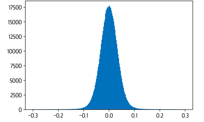
Meaning INT8 uses ¼ the memory of FP32. This small value range means:
- FP32 precision is not necessary
- Quantization noise is small
- Accuracy loss is minimal
This is why transformer models (BERT, DistilBERT, GPT-style models) tolerate INT8 quantization well.
There are 3 main quantization strtategies —
- Dynamic Quantization — Weights quantized ahead of time, Activations quantized at runtime, Easiest to apply (1 line of code), Best for transformers (NLP)
- Static Quantization — Quantization is computed in advance using calibration data, Better accuracy than dynamic, Requires representative dataset, Adds pipeline complexity
- Quantization-aware training — Simulates quantization during training, Best accuracy, Most complex, Used in cases where accuracy drop is unacceptable
from torch.quantization import quantize_dynamic

model_quantized = quantize_dynamic(
    model, {nn.Linear}, dtype=torch.qint8
)
Only linear layers are quantized — this is standard practice and provides most of the speedup.
Using DistilBERT:
- Before quantization:
Model size ≈ 256 MB
Latency ≈ 26 ms - After INT8 quantization:
Model size ≈ 132 MB
Latency ≈ 12.5 ms
Accuracy drop ≈ negligible (0.876 after quantization)
Quantization nearly halved the latency while maintaining accuracy and reducing model size by nearly 50%.
Quantization is one of the simplest yet most impactful optimizations for transformer-based NLP models. By converting FP32 values into lightweight INT8 integers, we can achieve:
- massive speedups
- dramatic memory reductions
- minimal accuracy loss
- easy integration into existing pipelines
As transformers continue to power modern NLP systems, quantization will remain a cornerstone optimization technique — enabling real-time inference on everything from cloud CPUs to edge devices.
Making Models Sparser with Weight Pruning
The main idea behind pruning is to gradually remove weight connections during training such that the model becomes progressively sparser. The resulting pruned model has a smaller number of nonzero parameters which can then be stored in a compact sparse matrix format. Pruning can also be combined with quantization to obtain further compression.

The way most weight pruning methods work is to calculate a matrix S of importance scores and then select the top k percent of weights by importance. k act as a new hyper parameter to control the amount of sparsity in the model that is the proportion of weights that are zero valued. Lower values of k correspond to sparser matrices. From these scores we can then define a mask matrix M that masks the weights W during the forward pass with some input x and effectively creates a sparse network of activations a

To determine which weights should be eliminated and how should the remaining weights be adjusted for best performance and how can such network pruning be done in computationally efficient way.
Magnitude Pruning — It calculated the scores according to the magnitude of the weights and then derive the masks from M = Top K(S). We apply magnitude pruning in iterative fashion by first training the model to learn which connections are important and pruning the weights of least importatnce. The sparse model is then retrained and the process repeated until the desired sparsity is reached.
But at every step we need to train the model to convergence. For this reason it is generally better to gradually increase the initial sparsity to a final value after some number of steps N. One problem with magnitude pruning is that it is really designed for pure supervised learning where the importance of each weight is directly related to the task in hand.
Movement Pruning — The basic idea behind movement pruning is to gradually remove weights during fine tuning such that the model becomes progressively sparser. The weights and scores are learned during fine tuning instead of derived directly from the weights the scores in movement running are arbitrary and are learned through gradient descent like any other neural network parameter.
Magnitude Pruning produces two clusters of weights while movement pruning produces a smoother distribution
References:
- https://corp.roblox.com/newsroom/2020/05/scaled-bert-serve-1-billion-daily-requests-cpus
- https://arxiv.org/abs/1909.02027 — An Evaluation Dataset for Intent Classification and Out-of-Scope Prediction
- Natural Language Processing with Transformers : Building Language Applications with Hugging Face — Lewis Tunstall, Leandro Von Werra & Thomas Wolf